As SciPy is open source, it has a very active and vibrant community of developers due to which there are enormous number of modules present for a vast amount of scientific applications and calculations available with SciPy. Some of the complex mathematical operations which can be performed with SciPy are:
- Interpolation
- Integration
- Optimization
- Image processing
- Statistics
- Special function calculations etc.
SciPy can be compared to most command and standard libraries like GSL library for C++ and Matlab. As SciPy is built on top of NumPy package, these two packages can be integrated completely as well. If you can think of a mathematical operation which needs to be done, make sure you check SciPy library before you implement that module on your own because in most cases, SciPy have all the operations for you fully implemented already.
Install SciPy Library
Let’s install SciPy library before we move to the actual examples and concepts. There are two ways to install this package. First one includes using the Python package manager, pip:
The second way relates to Anaconda, we can install the package as:
Once the library is installed, we can import it as:
Finally, as we will be using NumPy as well (It is recommended that for all NumPy operations, we use NumPy directly instead of going through the SciPy package):
It is possible that in some cases, we will also like to plot our results for which we will use the Matplotlib library. Perform the following import for that library:
I will be using the Anaconda manager for all the examples in this lesson. I will launch a Jupyter Notebook for the same:

Now that we are ready with all the import statements to write some code, let’s start diving into SciPy package with some practical examples.
Working with Polynomial Equations
We will start by looking at simple Polynomial equations. There are two ways with which we can integrate Polynomial functions into our program. We can make use of poly1d class which makes use of coefficients or the roots of a polynomial for initialising a polynomial. Let’s look at an example:
first_polynomial = poly1d([3, 4, 7])
print(first_polynomial)
When we run this example, we will see the following output:
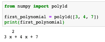
Clearly, the polynomial representation of the equation is printed as the output so that the result is pretty easy to understand. We can perform various operations on this polynomial as well, like square it, find its derivative or even solve it for a value of x. Let’s try doing all of these in the next example:
print(first_polynomial * first_polynomial)
print("Derivative of Polynomial: n")
print(first_polynomial.deriv())
print("Solving the Polynomial: n")
print(first_polynomial(3))
When we run this example, we will see the following output:
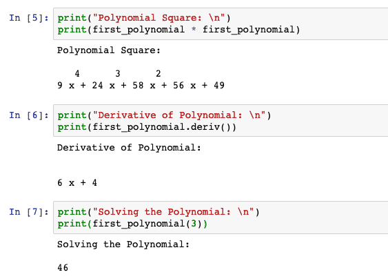
Just when I was thinking that this is all we could do with SciPy, I remembered that we can integrate a Polynomial as well. Let’s run a final example with Polynomials:
print(first_polynomial.integ(1))
The integer we pass tells the package how many times to integrate the polynomial:

We can simply pass another integer which tells the package how many times to integrate this polynomial.
Solving Linear Equations
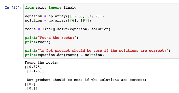
It is even possible to solve linear equations with SciPy and find their roots, if they exist. To solve linear equations, we represent the set of equations as NumPy arrays and their solution as a separate NumPy arrays. Let’s visualise it with an example where we do the same and make use of linalg package to find the roots of the equations, here are the equations we will be solving:
3x + 7y = 9
Let’s solve the above equations:
equation = np.array([[1, 5], [3, 7]])
solution = np.array([[6], [9]])
roots = linalg.solve(equation, solution)
print("Found the roots:")
print(roots)
print("n Dot product should be zero if the solutions are correct:")
print(equation.dot(roots) – solution)
When we run the above program, we will see that the dot product equation gives zero result, which means that the roots which the program found were correct:
Fourier Transformations with SciPy
Fourier Transformations helps us to express a function as separate components that make up that function and guides us about the way through which we can recombine those components to get the original function back.
Let’s look at a simple example of Fourier Transformations where we plot the sum of two cosines using the Matplotlib library:
# Number of sample points
N = 500
# sample spacing
T = 1.0 / 800.0
x = np.linspace(0.0, N*T, N)
y = np.cos(50.0 * 2.0* np.pi * x) + 0.5 * np.cos(80.0 * 2.0 * np.pi * x)
yf = fft(y)
xf = np.linspace(0.0, 1.0/(2.0 * T), N//2)
# matplotlib for plotting purposes
import matplotlib.pyplot as plt
plt.plot(xf, 2.0/N * np.abs(yf[0:N//2]))
plt.title(‘Info’)
plt.ylabel(‘Y axis’)
plt.xlabel(‘X axis’)
plt.grid()
plt.show()
Here, we started by constructing a sample space and cosine equation which we then transformed and plotted. Here is the output of the above program:
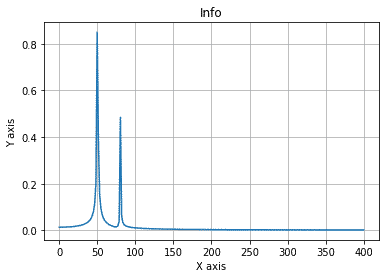
This is one of the good example where we see SciPy being used in a complex mathematical equation to visualise things easily.
Vectors and Matrix with SciPy
Now that we know a lot of things which SciPy is capable of, we can be sure that SciPy can also work with Vectors and Matrix. The matrices are an important part of linear algebra as matrices is something we use to represent Vector mappings as well.
Just like we looked at solving linear equations with SciPy, we can represent vectors with np.array() functions. Let’s start by constructing a matrix:
print(my_matrix)
Here is the output of the above snippet:

Whenever we talk about matrices, we always talk about Eigenvalues and Eigenvectors. To put in simple words, Eigenvectors are the vectors which, when multiplied with a matrix, do not change their direction, as opposed to most of the vectors. This means that even when you multiply an Eigenvectors with a matrix, there exists a value (or eigenvalue) which is one of the factor of the multiplication. This means:
In above equation, A is the matrix, λ is the Eigenvalue and x is the Vector. Let’s write a simple code snippet to find the Eigenvalues for a given Vector:
print(vector[:, 0])
print(vector[:, 1])
print(linalg.eigvals(my_matrix))
When we run this example, we will see the following output:

Calculating Matrix Determinant
The next operation we will carry out with SciPy is to calculate the determinant of a 2-dimensional matrix. We will reuse the matrix we used in the last code snippet here:
When we run this example, we will see the following output:

Conclusion
In this lesson, we looked at a lot of good examples where SciPy can help us by carrying out complex mathematical computations for us with an easy to use API and packages.
