Overall, we will cover three main topics in this lesson:
- What are Tensors and TensorFlow
- Applying ML algorithms with TensorFlow
- TensorFlow use-cases
TensorFlow is an excellent Python package by Google which makes good use of dataflow programming paradigm for highly optimized mathematical computations. Some of the features of TensorFlow are:
- Distributed computation capability which makes managing data in large sets easier
- Deep learning and neural network support is good
- It manages complex mathematical structures like n-dimensional arrays very efficiently
Due to all of these features and the range of machine learning algorithms TensorFlow implements, makes it a production scale library. Let’s dive into concepts in TensorFlow so that we can make our hands dirty with code right after.
Installing TensorFlow
As we will be making use of Python API for TensorFlow, it is good to know that it works with both Python 2.7 and 3.3+ versions. Let’s install TensorFlow library before we move to the actual examples and concepts. There are two ways to install this package. First one includes using the Python package manager, pip:
The second way relates to Anaconda, we can install the package as:
Feel free to look for nightly builds and GPU versions on the TensorFlow official installation pages.
I will be using the Anaconda manager for all the examples in this lesson. I will launch a Jupyter Notebook for the same:

Now that we are ready with all the import statements to write some code, let’s start diving into SciPy package with some practical examples.
What are Tensors?
Tensors are the basic data structures used in Tensorflow. Yes, they are just a way to represent data in deep learning. Let’s visualise them here:
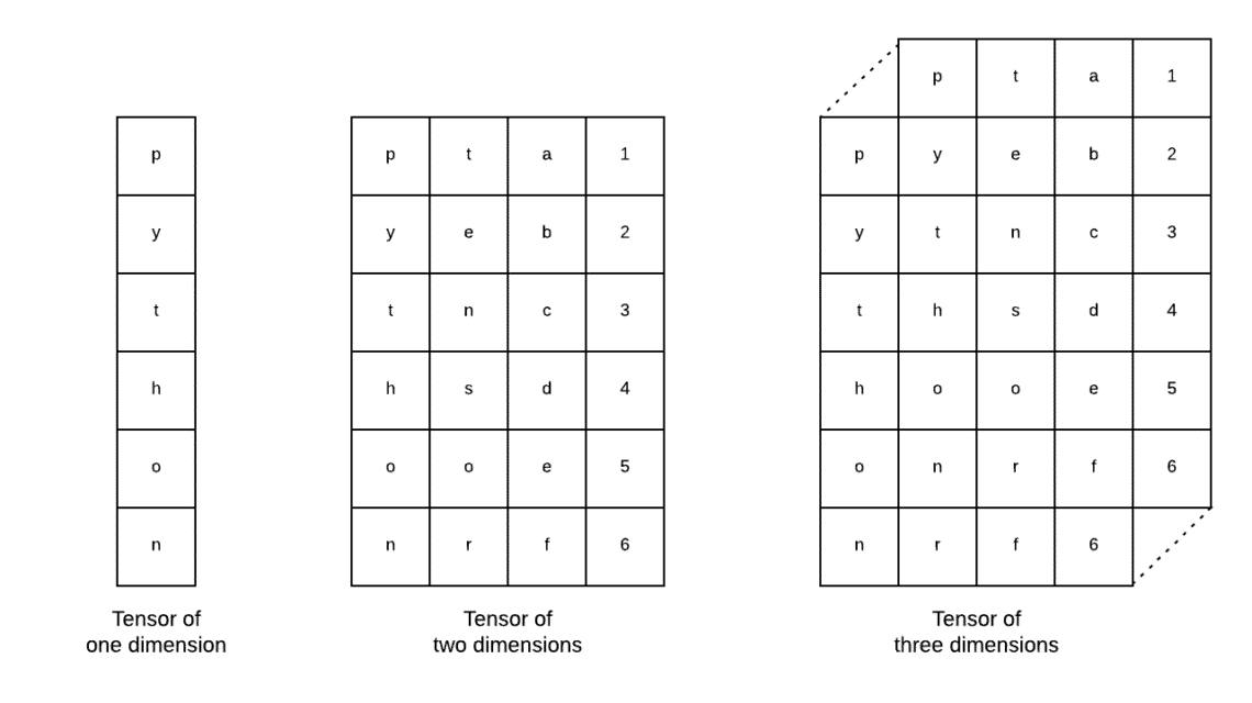
As described in the image, tensors can be termed as n-dimensional array which allows us to represent data in a complex dimensions. We can think of each dimension as a different feature of data in deep learning. This means that Tensors can grow out to be quite complex when it comes to complex datasets with a lot of features.
Once we know what Tensors are, I think it is quite easy to derive what happens in TensorFlow. That terms means how tensors or features can flow in datasets to produce valuable output as we perform various operations upon it.
Understanding TensorFlow with Constants
Just as we read above, TensorFlow allows us to perform machine learning algorithms on Tensors to produce valuable output. With TensorFlow, designing and training Deep Learning models is straight forward.
TensorFlow comes with building Computation Graphs. Computation Graphs are the data flow graphs in which mathematical operations are represented as nodes and data is represented as edges between those nodes. Let us write a very simple code snippet to provide a concrete visualisation:
x = tf.constant(5)
y = tf.constant(6)
z = x * y
print(z)
When we run this example, we will see the following output:
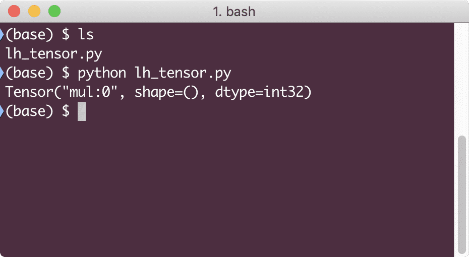
Why is the multiplication wrong? That wasn’t what we expected. This happened because this is not how we can perform operations with TensorFlow. First, we need to start a session to get the computation graph working,
With Sessions, we can encapsulate the control of operations and state of Tensors. This means that a session can also store the result of a computation graph so that it can pass that result to the next operation in the order of execution of the pipelines. Let’s create a session now to get the correct result:
session = tf.Session()
# Provide the computation to session and store it
result = session.run(z)
# Print the result of computation
print(result)
# Close session
session.close()
This time, we obtained the session and provided it with the computation it needs to run on the nodes. When we run this example, we will see the following output:

Although we received a warning from TensorFlow, we still got the correct output from the computation.
Single-element Tensor Operations
Just like what we multiplied two constant Tensors in the last example, we have many other operations in TensorFlow which can be performed on single elements:
- add
- subtract
- multiply
- div
- mod
- abs
- negative
- sign
- square
- round
- sqrt
- pow
- exp
- log
- maximum
- minimum
- cos
- sin
Single-element operations means that even when you provide an array, the operations will be done on each of the element of that array. For example:
import numpy as np
tensor = np.array([2, 5, 8])
tensor = tf.convert_to_tensor(tensor, dtype=tf.float64)
with tf.Session() as session:
print(session.run(tf.cos(tensor)))
When we run this example, we will see the following output:

We understood two important concepts here:
- Any NumPy array can be easily converted into a Tensor with the help of convert_to_tensor function
- The operation was performed on each of the NumPy array element
Placeholders and Variables
In one of the previous sections, we looked at how we can use Tensorflow constants to make computational graphs. But TensorFlow also allows us to take inputs on the run so that computation graph can be dynamic in nature. This is possible with the help of Placeholders and Variables.
In actual, Placeholders do not contain any data and must be provided valid inputs during runtime and as expected, without an input, they will generate an error.
A Placeholder can be termed as an agreement in a graph that an input will surely be provided at runtime. Here is an example of Placeholders:
# Two placeholders
x = tf. placeholder(tf.float32)
y = tf. placeholder(tf.float32)
# Assigning multiplication operation w.r.t. a & b to node mul
z = x * y
# Create a session
session = tf.Session()
# Pass values for placehollders
result = session.run(z, {x: [2, 5], y: [3, 7]})
print(‘Multiplying x and y:’, result)
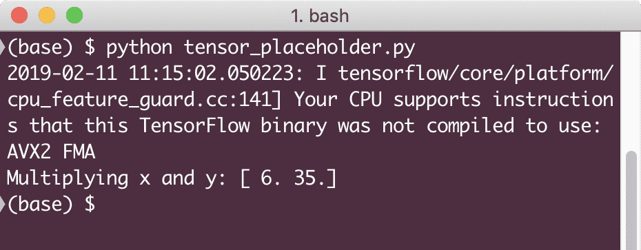
When we run this example, we will see the following output:
Now that we have knowledge about Placeholders, let’s turn our eye towards Variables. We know that output of an equation can change for same set of inputs over time. So, when we train our model variable, it can change its behaviour over time. In this scenario, a variable allows us to add this trainable parameters to our computational graph. A Variable can be defined as following:
In above equation, x is a variable which is provided its initial value and the data-type. If we do not provide the datatype, it will inferred by TensorFlow with its initial value. Refer to TensorFlow data types here.
Unlike a constant, we need to call a Python function to initialize all the variables of a graph:
session.run(init)
Make sure to run the above TensorFlow function before we make use of our graph.
Linear Regression with TensorFlow
Linear Regression is one of the most common algorithms used to establish a relationship in a given continuous data. This relationship between the coordinate points, say x and y, is called a hypothesis. When we talk about Linear Regression, the hypothesis is a straight line:
Here, m is the slope of the line and here, it is a vector representing weights. c is the constant coefficient (y-intercept) and here, it represents the Bias. The weight and bias are called the parameters of the model.
Linear regressions allows us to estimate the values of weight and bias such that we have a minimum cost function. Finally, the x is the independent variable in the equation and y is the dependent variable. Now, let us start building the linear model in TensorFlow with a simple code snippet which we will explain:
# Variables for parameter slope (W) with initial value as 1.1
W = tf.Variable([1.1], tf.float32)
# Variable for bias (b) with initial value as -1.1
b = tf.Variable([–1.1], tf.float32)
# Placeholders for providing input or independent variable, denoted by x
x = tf.placeholder(tf.float32)
# Equation of Line or the Linear Regression
linear_model = W * x + b
# Initializing all the variables
session = tf.Session()
init = tf.global_variables_initializer()
session.run(init)
# Execute regression model
print(session.run(linear_model {x: [2, 5, 7, 9]}))
Here, we did just what we explained earlier, let’s summarise here:
- We started by importing TensorFlow into our script
- Create some variables to represent the vector weight and the parameter bias
- A placeholder will be needed to represent the input, x
- Represent the linear model
- Initialize all the values needed for the model
When we run this example, we will see the following output:
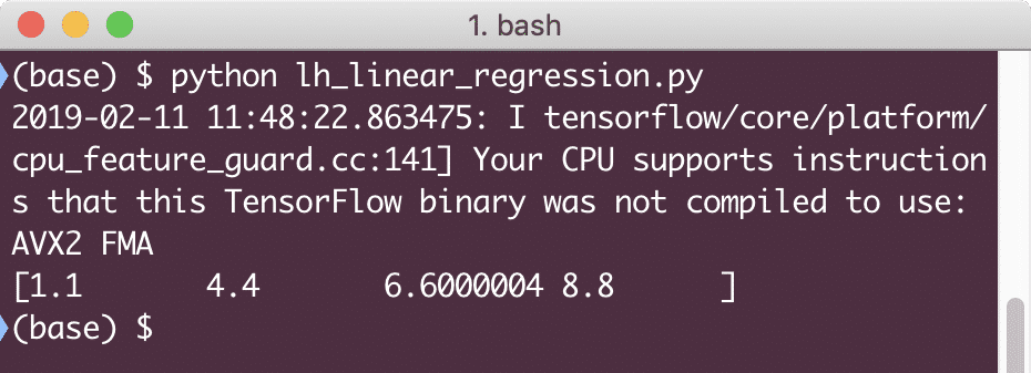
The simple code snippet just provides a basic idea about how we can build a regression model. But we still need to do some more steps to complete the model we built:
- We need to make our model self-trainable so that it can produce output for any given inputs
- We need to validate the output provided by the model by comparing it to the expected output for given x
Loss Function and Model Validation
To validate the model, we need to have a measure of how deviated current output is from the expected output. There are various loss functions which can be used here for validation but we will look at one of the most common methods, Sum of Squared Error or SSE.
The equation for SSE is given as:
Here:
- E = Mean Squared error
- t = Received Output
- y = Expected Output
- t – y = Error
Now, let us write a code snippet in continuance to the last snippet to reflect the loss value:
error = linear_model – y
squared_errors = tf.square(error)
loss = tf.reduce_sum(squared_errors)
print(session.run(loss, {x:[2, 5, 7, 9], y:[2, 4, 6, 8]}))
When we run this example, we will see the following output:

Clearly, the loss value is very low for the given linear regression model.
Conclusion
In this lesson, we looked at one of the most popular Deep learning and Machine learning package, TensorFlow. We also made a linear regression model which had very high accuracy.

